
使用深度学习进行艺术风格转换始于 Leon Gatys 等人于2015年发表的论文 A Neural Algorithm of Artistic Style,为普通照片 “赋予” 名画风格。由于其看上去不明觉厉的特性,在论文发表之后迅速得到了广泛关注,此后几年各种变种如雨后春笋般冒了出来,甚至诞生了大名鼎鼎的手机 app —— Prisma,下面就是一些通过 Prima 滤镜生成的图片。


本文主要参照这篇原始论文和书籍《Deep Learning with Python》对该项技术进行解读和实现。
原理
艺术风格转换的主要目的是将一张参考图片的风格应用到另一张原始图片上,最后的生成图片能既保留原始图片的大体内容,又展现出参考图片的风格。在本文的语境中,风格 (style) 不是指抽象主义、表现主义这类绘画流派的风格,而更多的是指狭义上一张图片的纹理、色彩、视觉模式等等。而内容 (content) 则指的是图片的宏观构造。
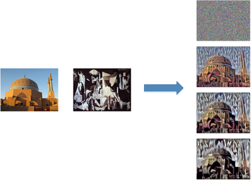
大致的流程是:输入为白噪声图像, 通过不断修正输入图像的像素值来优化损失函数,最终得到的图像即输出结果,如下图:
在对这些概念明了了之后,接下来要做的事情就很常规了:定义一个损失函数,然后优化。损失函数大致长这样:
loss=|参考图片的风格−生成图片的风格|styleloss+|原始图片的内容−生成图片的内容|contentlossloss=|参考图片的风格−生成图片的风格|styleloss+|原始图片的内容−生成图片的内容|contentloss
上式的意思是我们希望参考图片与生成图片的风格越接近越好,同时原始图片与生成图片的内容也越接近越好,这样总体损失函数越小则最终的结果越好。当然光有这个式子是不行的,计算机只认数字不认其他,所以这里的关键是如何用数学语言描述图片的内容和风格?
Content Loss
上文提到图片的内容主要指其宏观构造,而卷积神经网络的层数越深则越能提取图片中全局、抽象的信息,因而论文中使用卷积神经网络中高层激活函数的输出来定义图片的内容,那么衡量目标图片和生成图片内容差异的指标就是其欧氏距离 (即contentlosscontentloss):
Lcontent(C,G)=12∑i,j(a[l](C)ij−a[l](G)ij)2Lcontent(C,G)=12∑i,j(aij[l](C)−aij[l](G))2
其中a[l]ijaij[l]表示第ll层,第ii个featuremapfeaturemap的第jj个输出值。(C)(C)表示原始图片,(G)(G)表示生成图片,从上式可以看出比较的是二者在同一层激活函数的输出。
Style Loss
如何表示图片的风格呢? “风格” 本来就是个比较飘渺的概念,所以没有固定的表示方法,论文中采用的是同一隐藏层中不同featuremapfeaturemap之间的GramGram矩阵来表示风格,因而又称为 “风格矩阵” 。
设AA为m×nm×n的矩阵,则nn阶方阵GG为GramGram矩阵:
G=ATA=aT1aT2⋮aTn[a1a2⋯an]=aT1a1aT2a1⋮aTna1aT1a2aT2a2⋮aTna2⋯⋯⋱⋯aT1anaT2an⋮aTnanG=ATA=[a1Ta2T⋮anT][a1a2⋯an]=[a1Ta1a1Ta2⋯a1Tana2Ta1a2Ta2⋯a2Tan⋮⋮⋱⋮anTa1anTa2⋯anTan]
对于同一个隐藏层来说,不同的filterfilter会提取不同的特征,假设有NlNl个filterfilter,每个filterfilter输出的featuremapfeaturemap大小为MlMl(featuremapfeaturemap的height×widthheight×width),则这个隐藏层的输出可用一个矩阵Al∈RMl×NlAl∈RMl×Nl表示,则其GramGram矩阵Gl∈RNl×NlGl∈RNl×Nl代表了不同featuremapfeaturemap之间的相关性。 举例来说,假设一个filterfilter提取图片的红色特征,另一个filterfilter提取图片的蓝色特征,如果GramGram矩阵中这两个特征相关性高,则表示图片中同时出现了红色和蓝色,这在某种程度上可以代表其 “风格”,如下图:

在有了能定义风格的“风格矩阵”后,就能写出单个隐藏层的stylelossstyleloss了:
L[l]style(S,G)=14N2lM2l∑i,j(G[l](S)ij−G[l](G)ij)2Lstyle[l](S,G)=14Nl2Ml2∑i,j(Gij[l](S)−Gij[l](G))2
其中(S)(S)表示风格图片,(G)(G)表示生成图片,GijGij表示GramGram矩阵。如果使用多个隐藏层,则总体stylelossstyleloss就是:
Lstyle(S,G)=∑lw[l]⋅L[l]style(S,G)Lstyle(S,G)=∑lw[l]⋅Lstyle[l](S,G)
其中w[l]w[l]为各层的权重系数。
有了contentlosscontentloss和stylelossstyleloss后,总体 loss 就是其加权和:
Ltotal(C,S,G)=α⋅Lcontent(C,G)+β⋅Lstyle(S,G)Ltotal(C,S,G)=α⋅Lcontent(C,G)+β⋅Lstyle(S,G)
αα和ββ为超参数,用于调整Lcontent(C,G)Lcontent(C,G)和Lstyle(S,G)Lstyle(S,G)的相对比重。
实现
接下来我们来看论文中方法的具体实现,用的库是 Keras。论文作者 Gatys 等人没有从头训练一个CNN,而是使用了预训练 (pre-trained) 的 VGG-19 网络来对图片进行特征提取,这些特征可以帮助我们去衡量两个图像的内容差异和风格差异。大致流程如下:
将参考图片,原始图片,生成图片同时输入 VGG-19 网络,计算各个隐藏层的输出值。
定义并计算上文中描述的损失函数。
使用优化方法最小化损失函数。
首先读取图片,将所有图片转化为相似大小 (图片的高统一为 400px)。
import numpy as npfrom keras.applications import vgg19from keras.preprocessing.image import load_img, img_to_array

target_image_path = "original.jpg"style_reference_image_path = "style.jpg"width, height = load_img(target_image_path).size
img_height = 400img_width = int(width * img_height / height)def preprocess_image(image_path):  # 对图片预处理
    img = load_img(image_path, target_size=(img_height, img_width))
    img = img_to_array(img)
    img = np.expand_dims(img, axis=0)
    img = vgg19.preprocess_input(img)    return img
接下来导入 VGG-19 网络,其输入为三类图片 (参考图片,原始图片和生成图片) 的组合。
from keras import backend as K

target_image = K.constant(preprocess_image(target_image_path))
style_reference_image = K.constant(preprocess_image(style_reference_image_path))
combination_image = K.placeholder((1, img_height, img_width, 3))

input_tensor = K.concatenate([target_image,
                              style_reference_image,
                              combination_image], axis=0)

model = vgg19.VGG19(input_tensor=input_tensor, weights='imagenet', include_top=False)
定义contentlosscontentloss和stylelossstyleloss:
def content_loss(base, combination):
    return K.sum(K.square(combination - base))def gram_matrix(x):  # 用于计算 gram matrix
    #将表示深度的最后一维置换到前面,再flatten后就是上文中n*m的矩阵A
    features = K.batch_flatten(K.permute_dimension(x, (2, 0, 1)))
    gram = K.dot(features, K.transpose(features))    return gramdef style_loss(style, combination):
    S = gram_matrix(style)
    C = gram_matrix(combination)
    channels = 3
    size = img_height * img_width    return K.sum(K.square(S - C)) / (4. * (channels ** 2) * (size ** 2))
下图显示了 VGG-19 的结构:

上文提到图片的内容定义为卷积神经网络的高层激活函数输出,而风格则可以同时包含低层和高层输出,于是可以用最上面第5个 block 的输出计算contentlosscontentloss,所有5个 block 的输出计算stylelossstyleloss。
model = vgg19.VGG19(input_tensor=input_tensor, weights='imagenet', include_top=False)
outputs_dict = dict([(layer.name, layer.output) for layer in model.layers])  # 各隐藏层名称和输出的映射content_layer = 'block5_conv2'  # 第5个blockstyle_layers = ['block1_conv1',                'block2_conv1',                'block3_conv1',                'block4_conv1',                'block5_conv1']  # 所有5个block style_weight = 1.content_weight = 0.025loss = K.variable(0.)
layer_features = outputs_dict[content_layer]
target_image_features = layer_features[0, :, :, :]
combination_features = layer_features[2, :, :, :]
loss += content_weight * content_loss(target_image_features,
                                      combination_features)for layer_name in style_layers:
    layer_features = outputs_dict[layer_name]
    style_reference_features = layer_features[1, :, :, :]
    combination_features = layer_features[2, :, :, :]
    style = style_loss(style_reference_features, combination_features)
    loss += (style_weight * (style / len(style_layers)))
有了损失函数之后,最后一步就是优化。论文中使用的优化方法是 L-BFGS 算法,属于拟牛顿法之一,具有收敛速度快的特点。在这里我们使用 SciPy 中的 L-BFGS 算法,由于 Scipy 中的实现需要分别传入计算损失和梯度的函数,而分别计算这两个值会造成大量多余计算,所以这里建立一个 Evaluator 类,同时计算损失和梯度后由两个方法 [loss() 和 grads()]分别获得。
grads = K.gradients(loss, combination_image)[0]
fetch_loss_and_grads = K.function([combination_image], [loss, grads])class Evaluator(object):  # 建立一个类,同时计算loss和gradient
    def __init__(self):
        self.loss_value = None
        self.grads_values = None

    def loss(self, x):
        assert self.loss_value is None
        x = x.reshape((1, img_height, img_width, 3))
        outs = fetch_loss_and_grads([x])
        loss_value = outs[0]
        grad_values = outs[1].flatten().astype('float64')
        self.loss_value = loss_value
        self.grad_values = grad_values        return self.loss_value    def grads(self, x):
        assert self.loss_value is not None
        grad_values = np.copy(self.grad_values)
        self.loss_value = None
        self.grad_values = None
        return grad_values

evaluator = Evaluator()
经过了上面的铺垫后,就可以进行正式优化了,下面的代码迭代了20轮,并保存每一轮生成的图片。
from scipy.optimize import fmin_l_bfgs_bfrom scipy.misc import imsaveimport timedef deprocess_image(x): # 对生成的图片进行后处理
    x[:, :, 0] += 103.939
    x[:, :, 1] += 116.779
    x[:, :, 2] += 123.68
    x = x[:, :, ::-1]  # 'BGR'->'RGB'
    x = np.clip(x, 0, 255).astype('uint8')    return x

result_prefix = 'style_transfer_result'iterations = 20x = preprocess_image(target_image_path)
x = x.flatten()for i in range(1, iterations + 1):
    print('start of iteration', i)
    start_time = time.time()
    x, min_val, info = fmin_l_bfgs_b(evaluator.loss, x,
                                     fprime=evaluator.grads, maxfun=20)
    print('Current loss value: ', min_val)
    img = x.copy().reshape((img_height, img_width, 3))
    img = deprocess_image(img)
    fname = result_prefix + '_at_iteration_%d.png' % i
    imsave(fname, img)
    print('Image saved as', fname)
    print('Iteration %d completed in %ds' % (i, time.time() - start_time))
来看看效果:

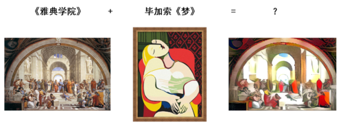
上面的例子中风格参考图片只用了一张,然而我们还可以使用多张图片来产生一种混搭风格,方法就是对每张图片的GramGram矩阵作加权平均。具体实现是要在stylelossstyleloss的定义中加入权重:
def style_loss(style, combination, weight):
    assert len(style) == len(weight)  # 图片数与权重数应相同
    S = [gram_matrix(st) * w for st, w in zip(style, weight)]
    S = K.sum(S, axis=0)
    C = gram_matrix(combination)
    channels = 3
    size = img_height * img_width    return K.sum(K.square(S - C)) / (4. * (channels ** 2) * (size ** 2))for layer_name in style_layers:
    layer_features = outputs_dict[layer_name]
    style_reference_features = layer_features[1, :, :, :]
    style_reference_features_2 = layer_features[2, :, :, :]
    combination_features = layer_features[3, :, :, :]
    style = style_loss([style_reference_features, style_reference_features_2, style_reference_features_3], combination_features, [0.2, 0.4, 0.4])
    loss += (style_weight * (style / len(style_layers)))


上面的 风格参考图片1为蒙克的《呐喊》,风格参考图片2为伦勃朗的《夜巡》,风格参考图片3为死亡金属专辑《Altar of Madness》的封面。其中《呐喊》被赋予的权重较低,所以其风格也少一些。
当然,这种风格转换的技术也有局限,其比较适合色调明亮,对比强烈的画作,如野兽派、立体派、后印象派等等,而若使用一些看上去相对“清淡”的画作为风格图片,则效果不明显。所以总的来说这种技术还是有很多探索空间的,下面以Github上的另一个实现作结:

完整代码
原文出处:https://www.cnblogs.com/massquantity/p/9621393.html