课程介绍
课程名称:Python3入门机器学习 经典算法与应用 入行人工智能
课程章节:5-1; 5-2; 5-3; 5-4
主讲老师:liuyubobobo
内容导读
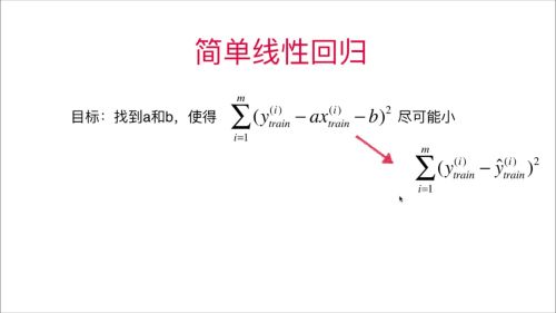
- 第一部分 实现简单线性回归法
- 第二部分 使用自己编写的一维线性回归代码
- 第三部分 向量化实现线性回归并测试效率
课程详细
- 第一部分 实现简单线性回归法
import numpy as np
import matplotlib.pyplot as plt

x = np.array([1., 2., 3., 4., 5.])
y = np.array([1., 3., 2., 3., 5.])

plt.scatter(x, y)
plt.axis([0, 6, 0, 6])
plt.show()

#第一步先计算x和y的均值
x_mean = np.mean(x)
y_mean = np.mean(y)

#求出分子和分母的和
num = 0.0
d = 0.0
for x_i, y_i in zip(x, y):
    num += (x_i - x_mean) * (y_i - y_mean)
    d += (x_i - x_mean) ** 2
a = num / d
b = y_mean - a * x_mean
y2 = x * a + b

plt.scatter(x,y)
plt.plot(x, y2, color="red")
plt.axis([0, 6, 0, 6])
plt.show()

x_predict = 6
y_predict = a * x_predict + b
y_predict
- 第二部分 使用自己编写的一维线性回归代码
from nike.SinmpleLinearRegression import SimpleLinearRegression1

linear_clf = SimpleLinearRegression1()

linear_clf.fit(x, y)
#SimpleLinearRegression1()
linear_clf.a_
linear_clf.b_

x_predict = np.array([0.5, 2.5, 5.5])
y_predict =linear_clf.predict(x_predict)
y_predict

plt.scatter(x,y)
plt.scatter(x_predict, y_predict,color="red")
# plt.plot(x, y2, color="red")
plt.axis([0, 6, 0, 6])
plt.show()

- 第三部分 向量化实现线性回归并测试效率
from nike.SinmpleLinearRegression import SimpleLinearRegression2
#fro循环
reg1 = SimpleLinearRegression1()
#向量化
reg2 = SimpleLinearRegression2()

x = np.arange(200000)
# np.random.randint(0,10)
y = 4 * x + 18

%%timeit
reg1.fit(x, y)
#31.2 s

%%timeit
reg2.fit(x, y)

#52.2 ms ms
二者运行时间相差至少600倍 由此可见向量化有多么强大
课程思考
向量化效率上非常之强大,以后数据哟啊是可以向量化的话,最好还是用矩阵计算,这几节课大多都是在进行公式推算,符号电脑打不出来,我是在笔记本上进行推算的,总了来说很奇妙,竟然可以用这种方式进行,原来这就是机器学习,我开始慢慢喜欢上机器学习了。
课程截图